  year gdp_growth
1 1990  4.1920510
2 1991  1.4383468
3 1992 -0.7994940
4 1993  0.3531973
5 1994  2.6327845
6 1995 4.4062165Time Series
Introduction to Time Series Analysis
Time series analysis involves analyzing data points collected or recorded at specific time intervals. It allows us to understand underlying patterns such as trend, seasonality, and cyclicity, which helps in making accurate forecasts. The two primary goals of time series analysis are to understand the underlying patterns in the data and to forecast future values. We will explore two popular methods The Holt-Winters method and the ARIMA model, using R to predict Kenya’s GDP Growth Rate for 2024.
The Holt-Winters Method
The Holt-Winters method, an extension of exponential smoothing, is designed to capture trends and seasonality in time series data. This method comes in two variants: additive and multiplicative, which cater to different types of seasonal patterns.
Additive Holt-Winters Method
The additive method is used when the seasonal variations are roughly constant over time. This approach involves three components: level, trend, and seasonality. The level represents the average value in the series, the trend captures the increase or decrease over time, and the seasonality accounts for repeating short-term cycles.
Multiplicative Holt-Winters Method
The multiplicative method is suitable when the seasonal variations change proportionally with the level of the series. Similar to the additive method, it also considers the level, trend, and seasonality, but in a way that the seasonal component multiplies with the level component.
The ARIMA Model
The ARIMA (AutoRegressive Integrated Moving Average) model is a versatile and widely used method for time series forecasting. It combines three key components namely:
Autoregressive (AR).
Integrated (I) .
Moving Average (MA).
Autoregressive (AR) Component
The AR component uses the relationship between an observation and a number of lagged observations. This helps in identifying and modeling the dependence of the current value on its previous values.
Integrated (I) Component.
The Integrated component involves differencing the observations to make the time series stationary. A stationary series has a constant mean and variance over time, which is a key requirement for ARIMA modeling.
Moving Average (MA) Component.
The MA component uses the dependency between an observation and a residual error from a moving average model applied to lagged observations. This helps in smoothing out the random fluctuations in the time series.
When to Use Holt-Winters and ARIMA Models
Choosing between the Holt-Winters method and the ARIMA model depends on the characteristics of the time series data at hand.
Holt-Winters Method
Use the Holt-Winters method when the time series data exhibits both a trend and seasonality. It is particularly effective when seasonal variations are either constant (additive) or proportional to the level of the series (multiplicative). For example, if Kenya’s GDP Growrh rate shows a consistent pattern of seasonal fluctuations along with a long-term growth trend, the Holt-Winters method would be a suitable choice.
ARIMA Model
The ARIMA model is best used when the time series data does not have a clear seasonal pattern but may have trends and other complexities. It is also useful when the data needs to be differenced to achieve stationarity. For example, if Kenya’s GDP data shows irregular trends without seasonal patterns, the ARIMA model can be adapted to capture these nuances.
Example to predict Kenya Annual GDP Growth Rate for 2024
Importing the data
Trends in Kenya GDP growth Rate
Quick Overview
1990s - Early 2000s
In the early 1990s, Kenya embarked on economic reforms aimed at liberalizing the economy and attracting foreign investment. However, the country faced challenges such as political instability and corruption, which hampered economic growth.Despite these challenges, the late 1990s saw a period of moderate GDP growth driven by sectors like agriculture, manufacturing, and services. Political reforms and improved governance in the late 1990s and early 2000s contributed to a more favorable investment climate, supporting economic expansion.
Mid-2000s - Pre-Financial Crisis (2005-2007)
The mid-2000s witnessed a period of relatively robust GDP growth, fueled by increased investment in infrastructure, telecommunications, and financial services. Government initiatives to promote private sector development and attract foreign direct investment (FDI) also supported economic expansion. Kenya economy benefited from favorable global conditions, including high commodity prices and strong demand for exports.
Global Financial Crisis (2008-2009)
The global financial crisis of 2008-2009 had a significant impact on Kenya economy, leading to a slowdown in GDP growth.Reduced demand for exports, declining remittances, and disruptions in global trade negatively affected key sectors like agriculture, tourism, and manufacturing. The crisis exposed vulnerabilities in Kenya financial sector and highlighted the importance of diversifying the economy and strengthening resilience to external shocks. The political instability that erupted in Kenya in 2007 and 2008, following disputed presidential elections, severely impacted the country’s GDP growth trajectory. Widespread violence and ethnic clashes paralyzed economic activities, disrupted supply chains, and caused significant damage to infrastructure and businesses.Investor confidence plummeted, leading to capital flight and a contraction in GDP growth
Post-Crisis Recovery (2010-2013)
Following the global financial crisis, Kenya experienced a period of recovery and resumed GDP growth, supported by government stimulus measures and renewed investor confidence. Infrastructure development projects, such as the construction of roads, ports, and energy facilities, played a crucial role in driving economic activity and creating employment opportunities. Kenya’s vibrant services sector, including telecommunications, banking, and information technology, emerged as a key driver of growth during this period.
2010s - Recent Years (2014-2023)
The 2010s saw mixed economic performance, with periods of strong growth interspersed with slowdowns and challenges. Factors such as political uncertainty, security concerns, and adverse weather conditions (e.g., droughts) posed headwinds to economic expansion.Nevertheless, Kenya continued to attract investment in sectors like real estate, energy, and infrastructure, supported by government initiatives to improve the business environment and promote entrepreneurship.
Code
library(dplyr)# for data manipulation
library(ggplot2)# for data visualization
library(forecast)# for time series analysis
p2 <- data %>%
  ggplot(aes(year, gdp_growth)) +
  geom_line(aes(color = "Economic Growth"), linewidth = 1, linetype = 1) +
  geom_smooth(aes(color = "Trend Line"), method = "lm", se = FALSE, linetype = 1, show.legend = TRUE) +
  ylim(-2, 10) + xlim(1990, 2027) + theme_bw() +
  labs(caption = "Source of the Data: Central Bank of Kenya",
       y = "GDP Growth Rate(%)",
       x = "Year") +
  theme(plot.title = element_text(colour = "black", size = 15, face = "bold"),
        axis.text.x = element_text(colour = "black"),
        axis.text.y = element_text(color = "black"),
        axis.title.x = element_text(face = "bold"),
        axis.title.y = element_text(face = "bold"),
        legend.position = "bottom", legend.title =element_blank()) +
  scale_color_manual(values = c("Economic Growth" = "blue", "Trend Line" = "red"),
                     labels = c("Economic Growth", "Trend Line"))
p2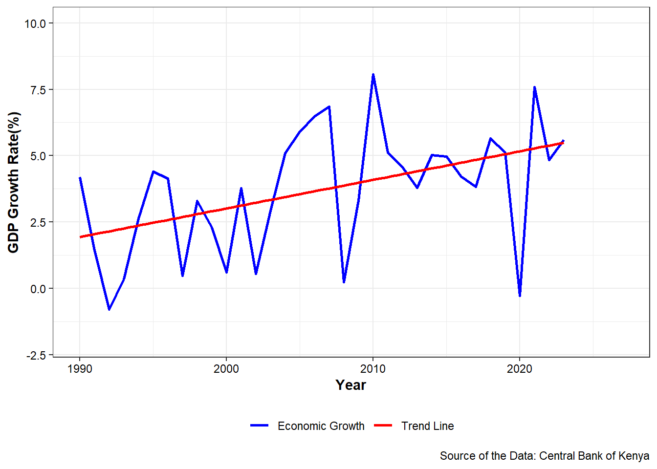
There seems to be a linear trend in the kenya gdp and no seasonality
Converting the Data to Timeseries
Code
data_timeseries <- ts(data$gdp_growth, start = 1990, frequency = 1)
data_timeseries
Time Series:
Start = 1990
End = 2023
Frequency = 1
[1] 4.1920510 1.4383468 -0.7994940 0.3531973 2.6327845 4.4062165
[7] 4.1468393 0.4749019 3.2902137 2.3053886 0.5996954 3.7799065
[13] 0.5468595 2.9324755 5.1042998 5.9066661 6.4724943 6.8507298
[19] 0.2322827 3.3069398 8.0584736 5.1211061 4.5686796 3.7978484
[25] 5.0201110 4.9677211 4.2135171 3.8379582 5.6479464 5.1141589
[31] -0.2727663 7.5904895 4.8466349 5.6000000Fitting the Model
Code
##(no seasonality, gamma is set as FALSE)
# Apply the additive Holt-Winters method
hw_additive <- HoltWinters(data_timeseries, seasonal = "additive",
                           gamma = F)

## Arima Model
arima <- auto.arima(data_timeseries)
Holt-Winters
Code
hw_additiveHolt-Winters exponential smoothing with trend and without seasonal component.
Call:
HoltWinters(x = data_timeseries, gamma = F, seasonal = "additive")
Smoothing parameters:
alpha: 0.581291
beta : 0.2717721
gamma: FALSE
Coefficients:
[,1]
a 5.4291790
b 0.2624884Level (a = 5.4291790): The current GDP growth rate is around 5.43%. This is the baseline value from which future growth is projected.
Trend (b = 0.2624884): The GDP growth rate is projected to increase by approximately 0.26% per year. This indicates a positive growth trend in the GDP growth rate.
Why These Parameters Matter
Alpha = 0.581291: The relatively high alpha value means the model is responsive to recent changes in GDP growth rate, allowing it to quickly adapt to new data.
Beta = 0.2717721: The moderate beta value indicates a stable trend estimation. The trend component is updated cautiously, which prevents overreacting to short-term fluctuations.
Gamma = FALSE: By setting gamma to FALSE, the model focuses solely on capturing the trend and level, which suits the nature of the data (no seasonality).
ARIMA
Code
arimaSeries: data_timeseries
ARIMA(0,1,1)
Coefficients:
ma1
-0.8241
s.e. 0.0916
sigma^2 = 5.141: log likelihood = -73.9
AIC=151.8 AICc=152.2 BIC=154.79The given ARIMA(0,1,1) model for the time series data_timeseries indicates that the series has been differenced once (indicated by the d=1term) to achieve stationarity, and a moving average component of order 1 (indicated by the q=1 term) is included
Model Prediction & Accuracy
Predicted value of Gdp Growth Rate for 2024 using Holtwinter Method
Code
forecast_additive Point Forecast Lo 80 Hi 80 Lo 95 Hi 95
2024 5.691667 1.842959 9.540376 -0.1944239 11.57776Predicted value of Gdp Growth Rate for 2024 using ARIMA Model
Code
forecat_arima Point Forecast Lo 80 Hi 80 Lo 95 Hi 95
2024 4.737344 1.831551 7.643138 0.2933165 9.181372Evaluating model
Histogram of Model Residuals
Code
# Plot the residuals for holtwinter method
hist(forecast_additive$residuals, xlab = "Residuals",
     main = "Histogram of Residuals(HoltWinter)", col = "red")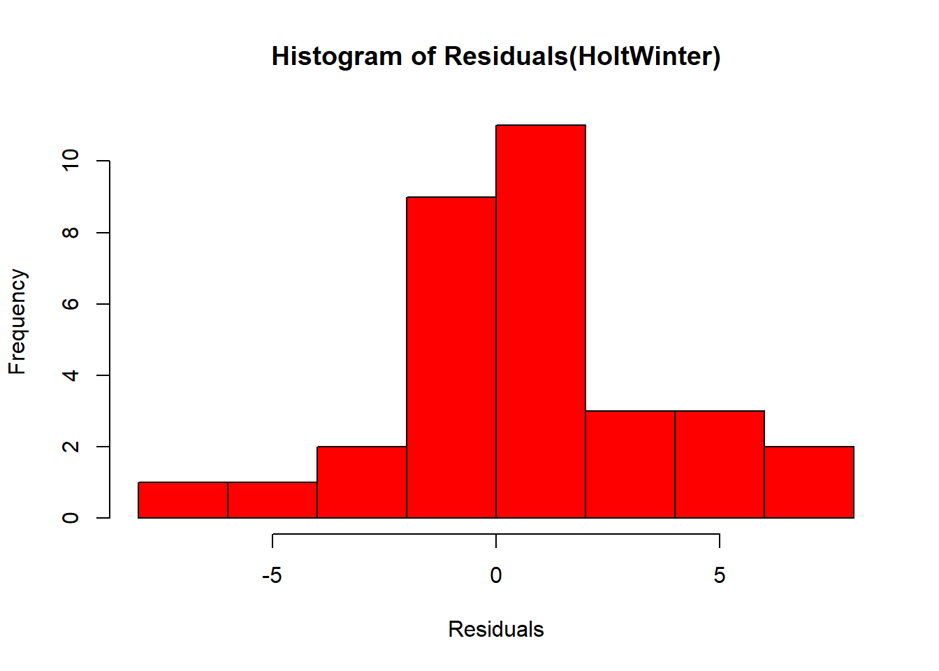
The plot shows that the distribution of forecast errors is roughly centred on zero
Ljung-Box test
Code
# Perform a Ljung-Box test on the residuals
Box.test(forecast_additive$residuals, type="Ljung-Box", lag = 20)
    Box-Ljung test

data:  forecast_additive$residuals
X-squared = 18.544, df = 20, p-value = 0.5516
Code
hist(arima$residuals,xlab = "Residuals",
     main = "Histogram of Residuals(ARIMA)", col = "blue")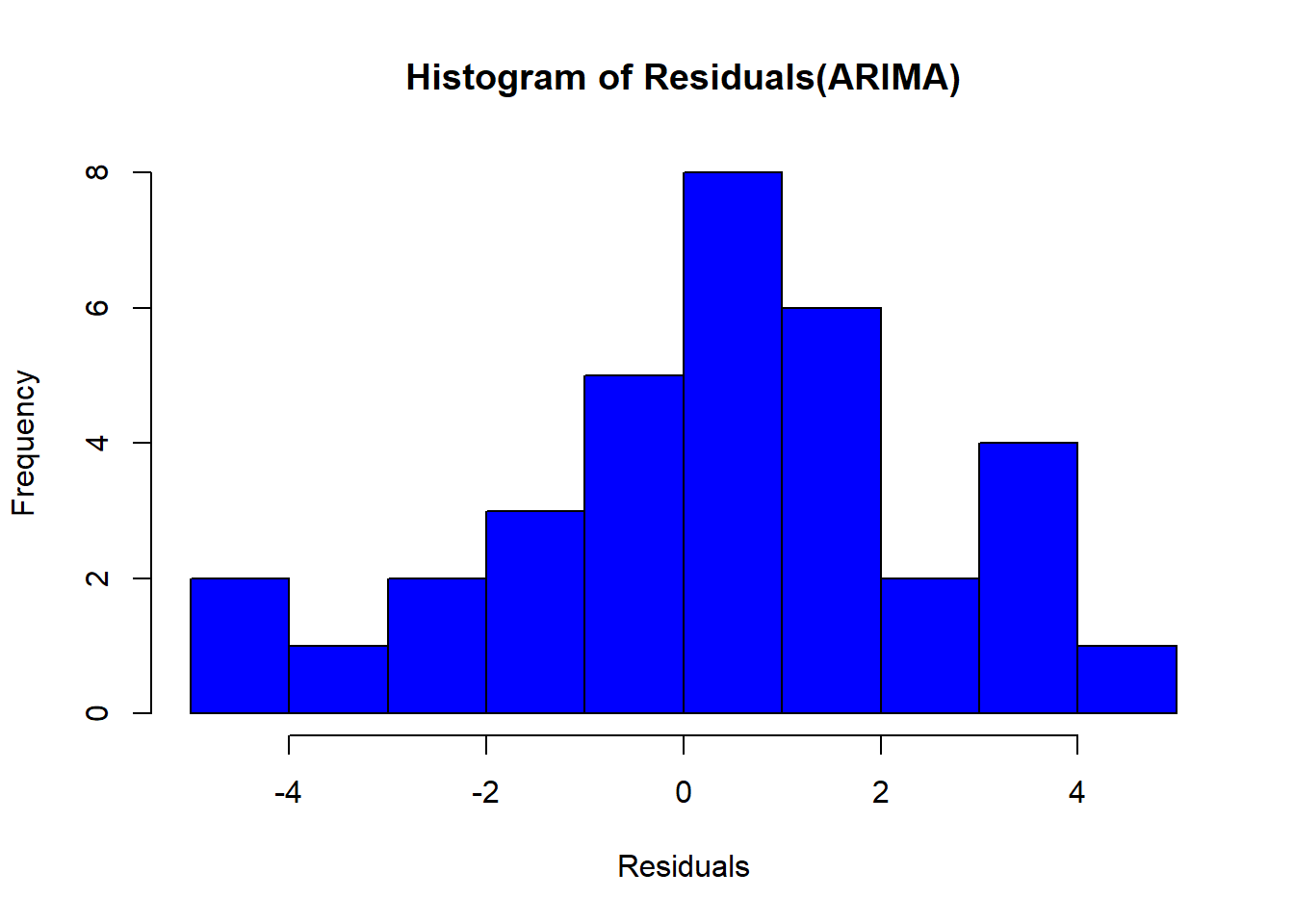
we may need to confirm the assumption using Ljung-Box test
Code
# Perform a Ljung-Box test on the residuals
Box.test(arima$residuals, type="Ljung-Box", lag = 20)
    Box-Ljung test

data:  arima$residuals
X-squared = 22.969, df = 20, p-value = 0.2903
The Ljung-Box test showed that there is little evidence of non-zero autocorrelations (p>0.05) in the in-sample forecast errors and the distribution of forecast errors seems to be normally distributed with mean zero. This suggests that the method provides an adequate predictive model Kenya GDP.